Exercise 3.12

Part (a). After introducing slack variables, we obtain the following standard form problem:

or rewritten equivalently in the matrix notation,

Note that $x=(0,0,2,6)$ is a basic feasible solution and can be used to start algorithm. Let accordingly $B(1)=3$ and $B(2)=4$. The corresponding basis matrix $B$ is the identity matrix $I$.

Part (b). To obtain the zeroth row of the initial tableau, we note that $c_B=0$ and, therefore, $c_B^{\prime }{x}_B=0$ and $\overline{c}=c$. Hence, we have the following initial tableau:

The reduced cost of $x_1$ is negative and we let that variable enter the basis. The pivot column is thus $u=-d_B=(1,1)$. We form the ratios $x_{B(1)}∕u_1=2$ and $x_{B(2)}∕u_2=6$; the smallest ratio corresponds to $l=1$. This determines the pivot element, which we indicate by an asterisk. The first basic variable $x_{B(1)}$, which is $x_3$, exits the basis. The new basis is given by $\overline{B}(1)=1$ and $\overline{B}(2)=4$. We multiply the pivot row by 2 and add it to the zeroth row. We subtract the pivot row from the last row. This leads us to the new tableau:

The corresponding basic feasible solution is $x^{(1)}=(2,0,0,4)$. With the curred tableau, the variable $x_2$ has a negative reduced cost. Thus, $x_2$ enters the basis next. The pivot column is $u=-d_B=(-1,2)$. Since $u_1<0$, we have $l=2$, and the second basic variable, $x_4$ exits the basis. The pivot element is again indicated by an asterisk. We add three halves of the pivot row to the zeroth row and half of the pivot row to the first row. After carrying out the necessary elementary row operations, we obtain the following new tableau:

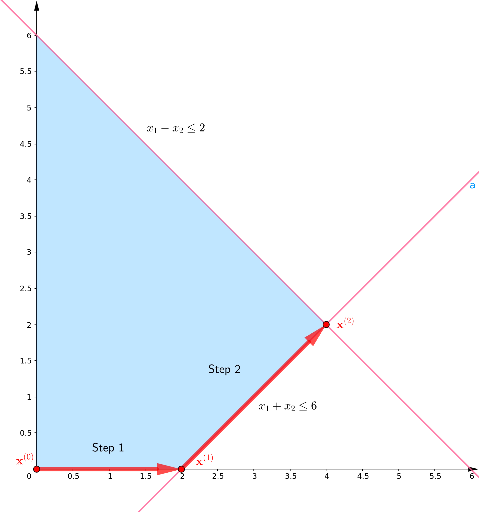
The corresponding basic feasible solution is $x^{(2)}=(4,2,0,0)$. In terms of the original variables $x_1,x_2$, we have moved to the point $(4,2)$. The optimality of this point is confirmed by observing that all reduced costs are non-negative.

Part (c). Red arrows indicate the path taken by the algorithm.